ECCV 2026

Whence the Voice?
Self-supervised Dual-source Audio-Visual Localisation via Selective Convergence

The MIx Group, School of Computer Science, University of Birmingham, UK
*Equal contribution
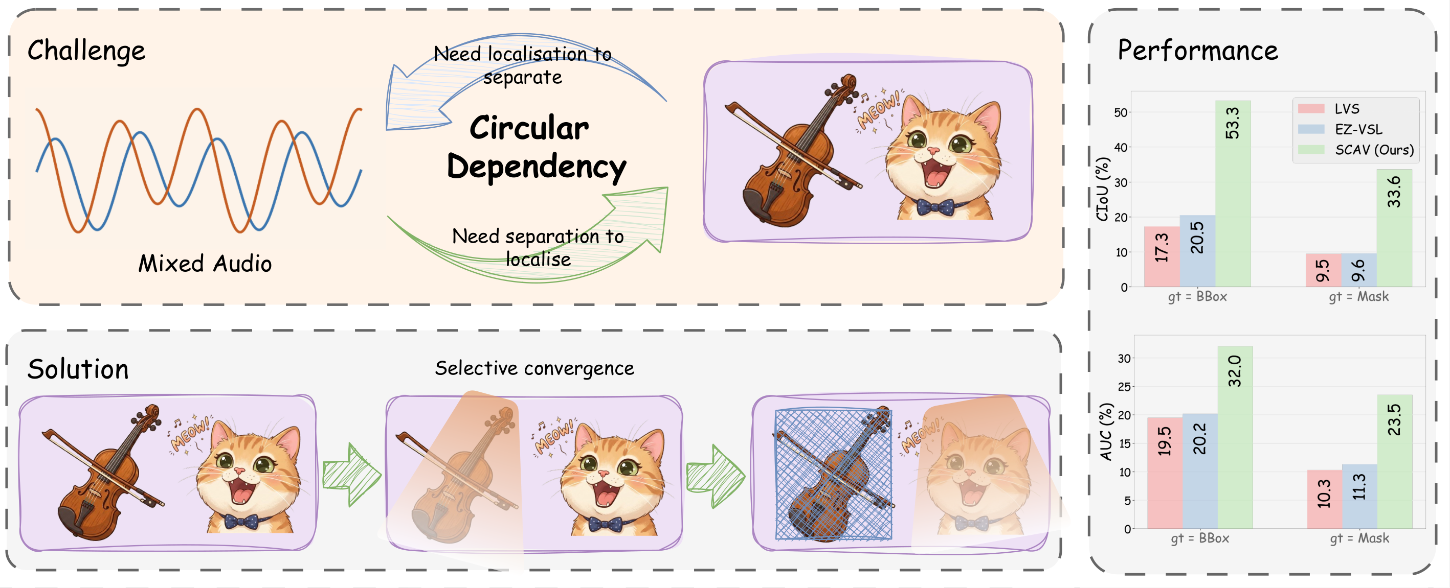
Overview of SCAV: the circular dependency, our two-stage framework, and performance.
The paradox & our idea. Localising mixed sources needs separated audio, while separating audio needs locations — a circular dependency. SCAV breaks it by exploiting selective convergence: the model first locks onto one source, then reveals the other.
Insight

Contrastive models naturally gravitate toward one source

When a contrastive audio-visual model is trained on mixed audio with two sounding objects, it does not split its attention evenly. It spontaneously commits to one source — the one it becomes biased toward.
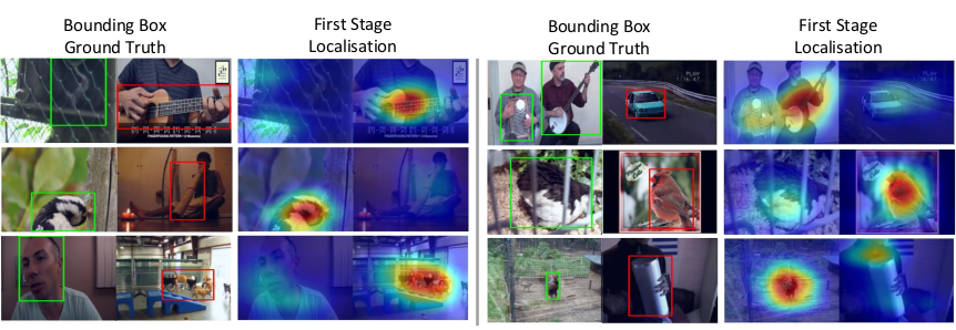
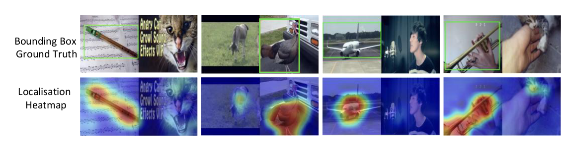
Examples of selective convergence: first-stage heatmaps concentrating on a single source.
Selective convergence in Stage 1. Given two ground-truth sources (green / red boxes), the first-stage heatmap concentrates on a single dominant source rather than both.
The model's bias is not a bug — it is the algorithm.
Method

A spatial prior breaks the circular dependency

SCAV turns the one-source bias into a feature, not a bug: it uses the dominant source as a spatial prior to progressively uncover the subdominant one.
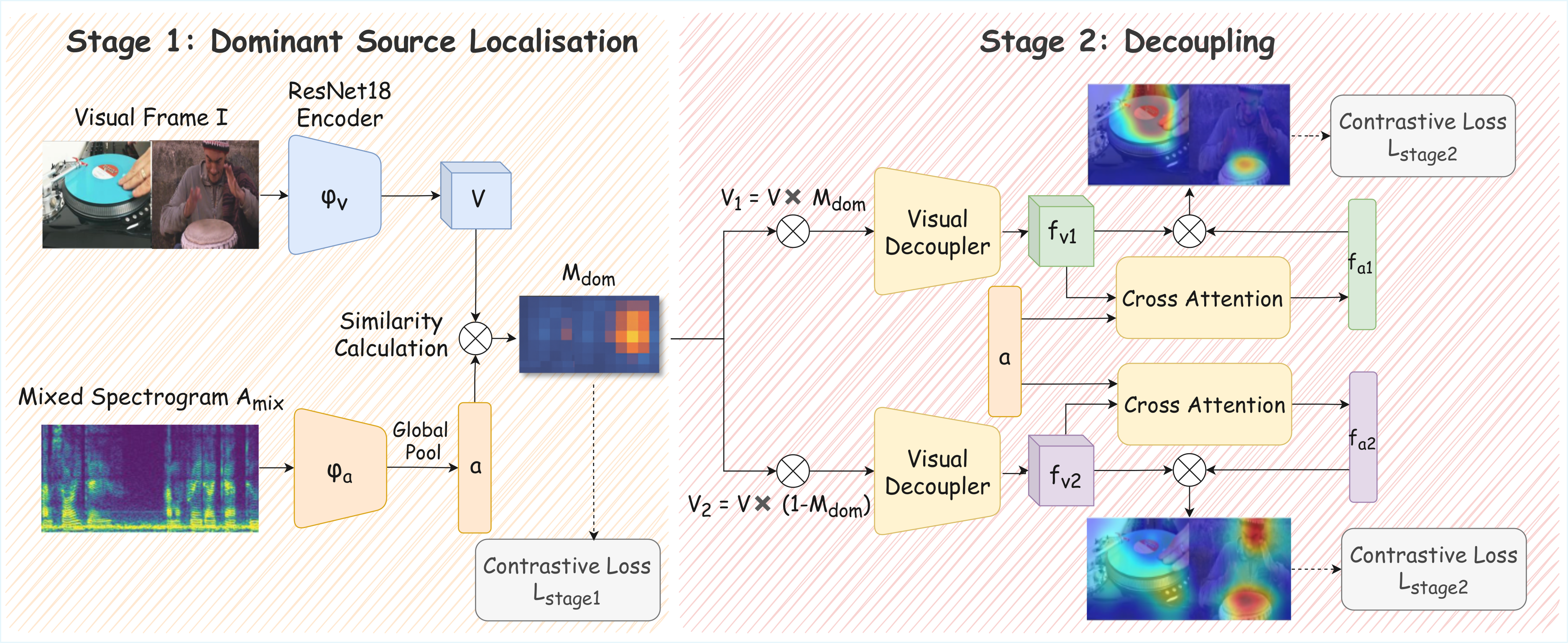
SCAV architecture: Stage 1 dominant-source localisation, Stage 2 progressive refinement.
SCAV architecture. Stage 1 (left) localises the dominant source via contrastive learning; Stage 2 (right) decouples visual and audio features to reveal the subdominant source.
Stage 1

Find the Dominant Source

Contrastive learning on the mixed audio drives the model to converge on a single source, yielding a clean spatial prior Mdom — no annotations required.

Stage 2

Reveal the Subdominant Source

Using Mdom as a prior, the model decouples the remaining audio-visual correspondence and localises the second source Msub in the same forward pass.

Dominant-source extraction (post-processing)
Post-processing algorithm for dominant source extraction.
Post-processing pipeline that extracts the dominant source region from the Stage 1 heatmap.
Results

Best self-supervised on every benchmark we tested

SCAV achieves the best performance among self-supervised methods across all benchmarks. All charts compare self-supervised methods only.

VGGSound-DuetMask — mask-based evaluation

Higher is better. Self-supervised methods only.

Bounding-box evaluation — CIoU@0.3

Self-supervised methods on MUSIC-Duet and VGGSound-Duet.
VGGSound-DuetMask Bounding-box

Qualitative Comparisons

Select a method to view its localisation results

Warmer colours = higher activation. SCAV produces focused, source-specific heatmaps; Mix-and-Localize collapses both sources into a single diffuse response.

Dataset

Bounding boxes lie — so we built a better benchmark

Existing benchmarks evaluate localisation against bounding-box annotations, which include substantial background and systematically inflate IoU. We introduce pixel-level segmentation masks for spatially-aligned evaluation.

DatasetYearTest SamplesAnnotation#Classes
MUSIC-Duet201817 Bounding Box11
MUSIC-Synthetic2020455Bounding Box15
VGGSound-Instruments2022446Segmentation Mask37
VGGSound-Duet20235,158 3,951 Bounding Box220
VGGSound-DuetMask (Ours)20253,951Segmentation Mask220

MUSIC-Duet counts are video-level; each video contains multiple annotated frames.   3,951 samples currently accessible; remaining videos are unavailable on YouTube.
Why bounding boxes mislead

Bounding boxes vs heatmaps comparison.
Boxes include backgroundGround-truth bounding boxes encompass substantial background beyond the actual sounding region — a guitar neck, the space around a violin, empty corners of a frame.
Metrics reward imprecisionMetrics against such boxes reward models that indiscriminately activate background pixels, paradoxically penalising precise localisation.
Masks fix the misalignmentOur pixel-level masks annotate only genuine sound-producing surfaces, enabling spatially-aligned evaluation.
Evaluation protocol: source-wise vs. frame-wise
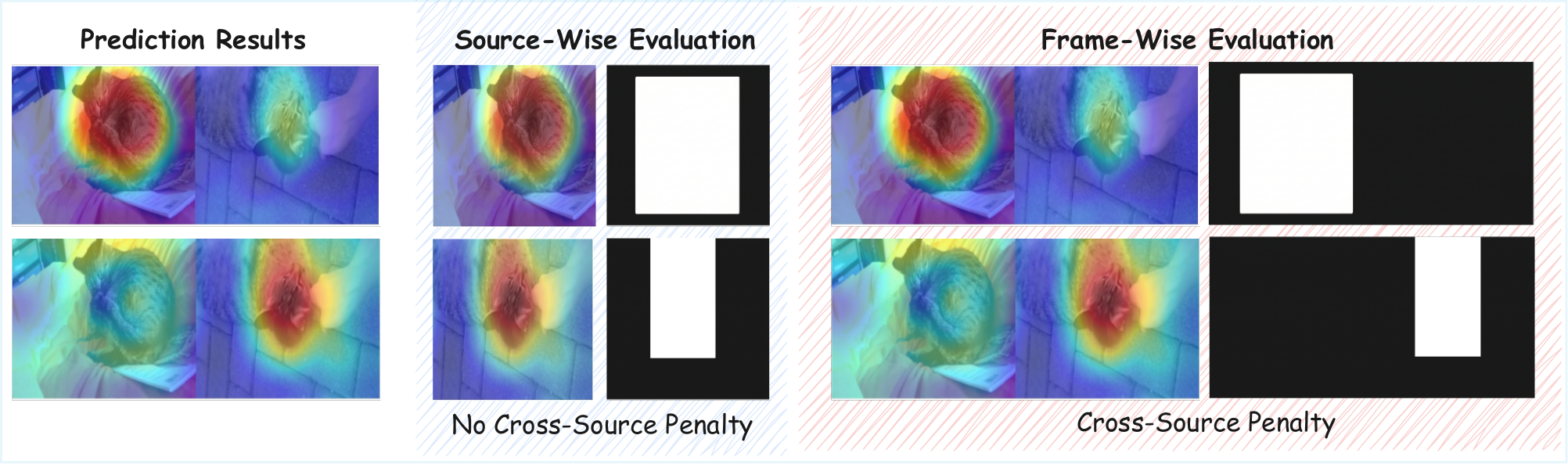
Source-wise vs frame-wise evaluation protocol.
Left: a synthetic dual-source test sample is formed by horizontally concatenating two single-source frames. Middle: source-wise evaluation crops each predicted heatmap to its designated half-frame — cross-source activations are never penalised, inflating all IoU-based metrics. Right: frame-wise evaluation (used in our paper) assesses each heatmap over the full $H\!\times\!2W$ frame against a zero-padded ground-truth mask, penalising any failure to suppress the non-target side.

The two protocols share the same numerator. Their denominators differ by $f_{\bar k}$, the number of activations on the opposite half-frame:

$$\underbrace{|\,\mathcal{B}_k \cup \mathcal{M}_k^{+}|}_{\text{frame-wise}} = \underbrace{|\,\hat{\mathcal{B}}_k \cup \mathcal{M}_k^{\mathrm{half}}|}_{\text{source-wise}} + f_{\bar{k}}$$

$$\mathrm{IoU}^{\,\text{src}}_{k} \;\ge\; \mathrm{IoU}^{\,\text{frame}}_{k}$$

Equality holds iff $f_{\bar k}=0$, i.e. the model produces zero activation on the opposite half. Source-wise evaluation therefore systematically inflates metrics whenever a model leaks activations across sources.

BibTeX

@inproceedings{hu2026scav,
  title     = {Whence the Voice? Self-supervised Dual-source Audio-Visual
               Localisation via Selective Convergence},
  author    = {Han Hu and Dongheng Lin and Yuqi Hou and Haotian Li and
               Hyung Jin Chang and Jianbo Jiao},
  booktitle = {European Conference on Computer Vision (ECCV)},
  year      = {2026}
}